Fisher equation
The Fisher equation in financial mathematics and economics estimates the relationship between nominal and real interest rates under inflation. It is named after Irving Fisher who was famous for his works on the theory of interest. In finance, the Fisher equation is primarily used in YTM calculations of bonds or IRR calculations of investments. In economics, this equation is used to predict nominal and real interest rate behavior. (Please note that economists generally use the Greek letter  as the inflation rate, not the constant 3.14159....)
Letting  denote the real interest rate,
  denote the nominal interest rate, and let denote the inflation rate, the Fisher equation is:

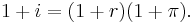
This is a linear approximation, but as here, it is often written as an equality:

The Fisher equation can be used in either ex-ante (before) or ex-post (after) analysis. Ex-post, it can be used to describe the real purchasing power of a loan:

Rearranged into an expectations augmented Fisher equation and given a desired real rate of return and an expected rate of inflation over the period of a loan,  , it can be used ex-ante version to decide upon the nominal rate that should be charged for the loan:

This equation existed before Fisher, but Fisher proposed a better approximation which is given below. The approximation can be derived from the exact equation:
Contents |
Derivation
Although time subscripts are sometimes omitted, the intuition behind the Fisher equation is the relationship between nominal and real interest rates, through inflation, and the percentage change in the price level between two time periods. So assume someone buys a $1 bond in period t while the interest rate is  . If redeemed in period, t+1, the buyer will receive
  dollars. But if the price level has changed between period t and t+1, then the real value of the proceeds from the bond is therefore

From here the nominal interest rate can be solved for.
 (1)
(1)
In expanded form, (1) becomes:


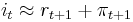
Assuming that both real interest rates and the inflation rate are fairly small, (perhaps on the order of several percent, although this depends on the application)  is much larger than
  and so can be dropped, giving the final approximation:
 .
.
More formally, this linear approximation is given by using two 1st order Taylor expansions, namely:
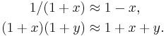
Combining these yields the approximation:

and hence 
Example
The market rate of return on the 4.25% UK government bond maturing on 8 March 2050 is 3.81% per year. Let's assume that this can be broken down into a real rate of exactly 2% and an inflation premium of 1.775% (no premium for risk, as government bond is considered to be "risk-free"):
1.02 × 1.01775 = (1 + 0.02) × (1 + 0.01775) = 1.0381
This article implies that you can ignore the least significant term in the expansion (0.02 × 0.01775 = 0.00035 or 0.035%) and just call the nominal rate of return 3.775%, on the grounds that that is almost the same as 3.81%.
At a nominal rate of return of 3.81% pa, the value of the bond is £107.84 per £100 nominal. At a rate of return of 3.775% pa, the value is £108.50 per £100 nominal, or 66p more.
The average size of actual transactions in this bond in the market in the final quarter of 2005 was £10 million. So a difference in price of 66p per £100 translates into a difference of £66,000 per deal.
Applications
The Fisher equation has important implications in the trading of inflation-indexed bonds, where changes in coupon payments are a result of changes in break-even inflation, real interest rates and nominal interest rates.
See also
References
- Barro, Robert J. (1997), Macroeconomics (5th ed.), Cambridge: The MIT Press, ISBN 0262024365.
- Fisher, Irving (1977) [1930]. The Theory of interest. Philadelphia: Porcupine Press. ISBN 0879918640.